4 Model Object

The Model Object within the MDL is intended to describe the mathematical and statistical properties of the model. MDL defines language elements that allow the user to code a wide variety of models and in a variety of ways. The Model Object is intended to specify the model independent of the target software which will be used for the task (estimation or simulation). The same model should be able to be used for a variety of tasks – estimation, simulation or optimal design without recoding. The Model Object should also be independent of the data – where possible we use enumerated types for categorical covariates and outcomes so that definition of the model is clear to any user regardless of the data used in a given task.

It should be noted however that MDL does not guide the user about whether the model that is defined is suitable for a given purpose or for any target software. The user is free to define any model, however they must also be aware that the specified model may not be useable with all target software.

As stated in the Introduction, the Model Object is intended to convey the mathematical and statistical definitions required to completely define the model. MDL used in defining the model is intended more as a descriptive language rather than a programmatic one. The Model Object is used in tasks by combining it with Data, Parameter and Task Properties objects, and defining tasks within the R script.

Currently defined blocks are IDV, COVARIATES, POPULATION_PARAMETERS, FUNCTIONS, VARIABILITY_LEVELS, STRUCTURAL_PARAMETERS, VARIABILITY_PARAMETERS, GROUP_VARIABLES, RANDOM_VARIABLE_DEFINITION, INDIVIDUAL_VARIABLES , MODEL_PREDICTION, DEQ, COMPARTMENT, OBSERVATION.

Which blocks within the Model Object are used for a particular model depends on the structure of that model. Blocks should not be left empty (although this is not a syntax error). It is good practice to structure and write the model to facilitate readability and understanding of the model. Simple statements that are clear and unambiguous are preferred to statements combining many actions into one line of code. Use of the MODEL_PREDICTION block is encouraged to make it clear what the final prediction is from the model prior to use in generation of the observation level.

In the current version of MDL, the variable names and parameter names in the STRUCTURAL_PARAMETERS and VARIABILITY_PARAMETERS blocks of the Model Object must be matched to those in the Data and Parameter objects. The MOG Object brings together the Data, Parameter, Model and Task Properties Objects to perform tasks, and at this stage it is assumed that the variable names match across objects.

The independence of the Data Object from the model means that the data referenced by the Data Object may be easily used with a different model without modification of the Data Object. Similarly, the independence of the Parameter Object from the model means that all the parameters related to modelling project e.g. describing a particular drug, may be stored in one place. Note that parameters defined in the Parameter Object must have unique names.

Unlike other MDL Objects, the Model Object does not use a DECLARED_VARIABLES block. Instead variables are declared when they are used within the IDV, COVARIATES, STRUCTURAL_PARAMETERS, VARIABILITY_PARAMETERS blocks. Particular care may be required for models defined using analytic equations (rather than via differential equations, compartments). In these models it may be necessary to declare inputs such as DOSE within the MODEL_PREDICTION block.

4.1 On interoperability

The primary focus of MDL in this release is translation to valid PharmML, rather than conversion to target software. The previous Public Release was primarily concerned with demonstrating interoperability across key software targets. In this version of MDL there may be features supported which are not supported by certain target software, but which are valid for model description and which generate valid PharmML. The aim is to widen the scope of models which can be encoded in MDL and generate PharmML, since the latter is required for uploading models to the DDMoRe repository. Translation of these models to target software will follow with updates to the interoperability framework converters.

The MDL-IDE should assist the user in ensuring that the models encoded are valid MDL (and as a consequence, also valid PharmML).

Models in MDL may be expressed in a number of ways, which may be influenced by a number of factors including which languages the user is familiar with for encoding models. Flexibility allows the user to encode models quickly in a common language (MDL) which can then be shared with others and mutually understood. This flexibility also facilitates encoding in a given target when that language construct does not have a parallel in other tools. However, we STRONGLY encourage the user to encode the majority of models in a way that will facilitate interoperability. Interoperability allows the user of the model to choose the best tool for the job, or at least the tools that they have available to them.

If the user follows certain conventions for coding then it will increase the chance that a given model is interoperable between target tools. These conventions will be highlighted in the subsequent sections, but users should pay particular attention to sections 4.7, 4.9 and 4.10 on definition of GROUP_VARIABLES defining fixed effects, INDIVIDUAL_VARIABLES defining the relationship between covariates (or GROUP_VARIABLES defined variables) and random effects and MODEL_PREDICTION using these parameters to calculate predictions for given inputs.

4.2 `IDV`

The IDV block defines the independent variable within the model. Typically this is TIME (or T for differential equations). An IDV block must be present in the Model Object.

The syntax is a simple variable declaration:

IDV{ <Independent variable name> }

4.3 `COVARIATES`

The COVARIATES block declares and defines covariates to be used in the GROUP_VARIABLES, INDIVIDUAL_VARIABLES and MODEL_PREDICTION blocks (see discussion of regressors below for use of covariates in the MODEL_PREDICTION block). Covariates listed in the COVARIATES block must be specified as use is covariate or use is catCov in the DATA_INPUT_VARIABLES block in the Data Object or defined in the POPULATION block of the Design Object. Covariate transformations may be specified within this block.

COVARIATES{
< Covariate name >
< Categorical covariate name > withCategories {< category1 >, < category2 >, … , < category_k >}
< Covariate name > = <simple transformation equation>
}

For categorical covariates, the categories defined in the COVARIATES block must match those specified for DATA_INPUT_VARIABLES with use is catCov – see the definition of the SEX covariate above.

An example COVARIATES block is shown below:

COVARIATES{
  WT
  SEX withCategories {female, male}
  logtWT = ln(WT/70)
}

In this example the withCategories prefix to the list of category names will be used to link to the values associated with these names in the Data Object.

The logtWT variable in the COVARIATES block may be used as the value for the cov attribute in the linear function in the INDIVIDUAL_VARIABLES block if WT follows the above rules for covariates.

Please also read about the specification of covariate models in sections 4.7 and 4.9.

The definition of covariates above assumes that the covariates are constant within individuals or vary only at occasion levels. It is also possible to define covariates that vary with the independent variable (typically time):

COVARIATES(type is idvDependent){
  WT
  logtWT = ln(WT/70)
}

Covariates which are defined as idvDependent should NOT be used in the type is linear definition of INDIVIDUAL_PARAMETERS.

4.4 `STRUCTURAL_PARAMETERS`

This block declares fixed effect parameters that define the structure of the model. There is no separator character in between variable names. The variable names do not need to be on separate lines, but it may be easier to read if they are presented in this way and it allows comments to be added to help communication

STRUCTURAL_PARAMETERS{
  < Variable name(s) of structural parameters >
}

For example:

STRUCTURAL_PARAMETERS {
  POP_CL
  POP_V
  POP_KA
  POP_TLAG
  BETA_CL_WT
  BETA_V_WT
} # end STRUCTURAL_PARAMETERS

4.5 `VARIABILITY_PARAMETERS`

Similar to the STRUCTURAL_PARAMETERS block, this block declares all the variability (including covariance, correlation and residual error) parameters (population parameter variability and other variability level parameters) used in the model. The variable names do not need to be on separate lines, but it may be easier to read if they are presented in this way and allows comments to be added to help communication

VARIABILITY_PARAMETERS{
<Variable name(s) of variability parameters>
}

For example:

VARIABILITY_PARAMETERS {
  PPV_CL
  PPV_V
  CORR_CL_V
  PPV_KA
  PPV_TLAG
  RUV_ADD
  RUV_PROP
} # end VARIABILITY_PARAMETERS

4.5.1 Residual Unexplained Variability

Residual variability is typically defined as a standard Normal distribution ~N(mean=0, var=1). The standard residual error models (see section 4.12.1) then define the parameters of that model e.g. additive and proportional which multiply the random N(0,1) variable. They can also define expressions involving parameters which define the residual error model. These parameters should be declared as VARIABILITY_PARAMETERS.

4.6 `VARIABILITY_LEVELS`

The VARIABILITY_LEVELS block defines the model hierarchy. Each variable should have attributes defining its level in the model hierarchy and variability type which is one of parameter or observation. DATA_INPUT_VARIABLES with use is dv and use is id are automatically identified as describing variability levels. Additional variables can be used to define variability levels by defining these as use is varLevel in DATA_INPUT_VARIABLES.

Typically, level = 1 is the level of each sample / experimental unit / observation. Additional levels of the hierarchy built on top of this. Typically in population models there is at least one additional level of variability – that of the individual (the experimental unit). Occasionally if modelling summary level data in a model-based meta-analysis, treatment arm may be used as the experimental unit and labelled in the DATA_INPUT_VARIABLES block as use is id.

The syntax is:

  VARIABILITY_LEVELS(reference = < ID | varLevel >){
      <Variable name> : { level = <number>, type is <parameter | observation>}
      ... # Additional levels of variability specified as above
  }

For example:

VARIABILITY_LEVELS(reference=ID){
  ID : { level=2, type is parameter }
  DV : { level=1, type is observation }
  }

If between occasion variability is required in the model then this should be specified here as a variability level between the observation and individual levels. In NONMEM occasion is typically specified as an additional layer of inter-individual variability which is defined conditionally on an occasion variable in the dataset. In MDL this is explicitly treated as a distinct level of variability.

VARIABILITY_LEVELS(reference=ID){
 ID : { level=3, type is parameter }
 OCC : { level=2, type is parameter }
 DV : { level=1, type is observation }
 }

Additional levels of variability are easily implemented by incrementing level = <number> with an associated DATA_INPUT_VARIABLE with use is varLevel. This facilitates definition of levels such as between trial random variability.

The distinction between type is observation and type is parameter will be used further in future versions of MDL to describe models where there are additional levels of hierarchy. For example, when describing differences between trials as a random effect or modelling population level differences; and at the observation level e.g. replicates of PD measurements at each time point, or multiple assays of a single sample. Specifying variability type allows extensibility for the future while retaining backwards compatibility.

When estimating model parameters using observed data, the DATA_INPUT_VARIABLE with use is id is the default “reference level of the model hierarchy (Gelman 2006). When using a Design Object, the reference level of the model hierarchy is likely to be implicit (subjects in a study arm) rather than explicit. Thus the need to specify reference = ID.

4.7 `GROUP_VARIABLES`

The GROUP_VARIABLES block can be used to specify group specific variables using parameters and fixed effect relationships between parameters and covariates. The INDIVIDUAL_VARIABLES block can then use these values in definition of the individual parameters by incorporating the random between individual variabilities defined in the RANDOM_VARIABLE_DEFINITION block(s).

Using the GROUP_VARIABLES block to define covariate relationships is not supported for parameter estimation in some target software since the equations defined in the GROUP_VARIABLES block are user defined. The MDL-IDE is not equipped to determine whether the defined relationships conform to linear relationships (after transformation) that have been shown to allow interoperability between software.

For this reason we suggest that definition of covariate dependent GROUP_VARIABLES is used only in cases where a reformulation to “linear or “linear after transformation relationships with covariates as defined in section 4.9 is not possible.

The GROUP_VARIABLES block is essential for defining relationships between structural parameters and covariates which are non-linear, even after transformation. For example to describe clearance across both adults and children a maturation model may be required. For example:

GROUP_VARIABLES{
  FSIZE = (WT/70)^0.75
  FAGE = if(AGE >= 20) then exp(BETA_CL_AGE*(AGE-20))
         else 1
  FMAT = 1/(1+(PCA/TM50)^(-HILL))
  GRP_CL = POP_CL * FSIZE * FAGE * FMAT
}

GRP_CL can then be used in the definition of individual variables within the INDIVIDUAL_VARIABLES block.

4.7.1 Defining model constants

Model constants (model variables with constant values) may be defined in MDL within the GROUP_VARIABLES block.

However, to ensure interoperability within the current SEE, constant values in the model should be defined as STUCTURAL_PARAMETERS and fixed to a value in the Parameter Object.

For models expressed as systems of differential equations (DEQ block), model variables can be set to constant values in the MODEL_PREDICTION block, but this may be computationally inefficient in the target software implementation.

4.8 `RANDOM_VARIABLE_DEFINITION`

The RANDOM_VARIABLE_DEFINITION block defines the distribution of the random effects to be used in construction of mixed effects models. The RANDOM_VARIABLE_DEFINITION block defines random variables in terms of parametric distributions.

It is assumed that all variables within the same block are defined for the same level of the model hierarchy. Separate RANDOM_VARIABLE_DEFINITION blocks should be used for each layer of the model hierarchy.The user specifies which level through the (level = <name of variable associated with this level> ) syntax following the RANDOM_VARIABLE_DEFINITION block name.

The following syntax is used to define random variables:

RANDOM_VARIABLE_DEFINITION( level = <VARIABILITY_LEVEL variable> ){
  <VARIABLE NAME > ~ <Distribution with arguments>
 }

The RANDOM_VARIABLE_DEFINITION block supports probability distributions as specified in the ProbOnto knowledge base (M. J. Swat, Grenon, and Wimalaratne 2016). Typically for definition of structural parameter and residual error random variability, Normal distributions will be used. The MDL distribution “Normal(…) maps to either ProbOnto Normal1 or Normal2 depending on the parameterisation:

MDL Name	Argument name	Argument Types	ProbOnto distribution
Normal	mean	Real	Normal1
	sd	Real
Normal	mean	Real	Normal2
	var	Real

This means that the user does not need to remember which ProbOnto distribution uses which parameterisation for this frequently used distribution.

An example of RANDOM_VARIABLE_DEFINTION for individual random effects is given below:

RANDOM_VARIABLE_DEFINITION( level = ID ) {
  ETA_CL  ~ Normal(mean = 0, sd = PPV_CL)
  ETA_V   ~ Normal(mean = 0, sd = PPV_V)
  ETA_KA  ~ Normal(mean = 0, sd = PPV_KA)
  ETA_TLAG ~ Normal(mean = 0, sd = PPV_TLAG)
} # end RANDOM_VARIABLE_DEFINITION

In the code above, ETA_CL, ETA_V, ETA_KA and ETA_TLAG vary with each new value of ID. These variables are normally distributed with mean = 0 and standard deviation defined by the variability parameters. The distribution can also be defined using variances.

In the example above, all random variability parameters are independent. To specify correlation or covariance between parameters, the user should specify either pairwise correlation or covariance between random variables or use a multivariate distribution. In contrast to the previous version of MDL where correlations and covariances were defined only in the Parameter Object, this version requires the user to specify correlations and covariances in the RANDOM_VARIABLE_DEFINITION block. This is to allow the Prior Object to define priors on parameters used in the Model Object.

The following syntax is used to define correlation or covariance:

:: {type is <correlation / covariance>,
  rv1 = <RANDOM_VARIABLE_DEFINITION variable>,
  rv2 = <RANDOM_VARIABLE_DEFINITION variable>,
  variable = <VARIABILITY_PARAMETERS parameter> }

Note the use of the “anonymous list using double colon “:: . This is used since we are assigning additional information to the variable defined in the VARIABILITY_PARAMETERS block.

For example (UseCase1):

:: {type is correlation, rv1=ETA_CL, rv2=ETA_V,
value=CORR_CL_V}

Alternatively, the user can specify multivariate distribution(s) for parameters to specify the joint distribution of multiple random variability parameters. To do this, the user must specify the type of parameters in the STRUCTURAL_PARAMETERS (if required) and VARIABILITY_PARAMETERS blocks. Typically for multivariate distributions, there may be a vector of mean values, and a matrix of correlations or covariances. We can then use these to define the multivariate distribution using ProbOnto definitions.

So if we assume that the random effects for CL, V and KA (ETA_CL, ETA_V and ETA_KA in the univariate case) come from a multivariate distribution then the distribution of the vector ETA_CL_V_KA is given as:

\[ETA\_ CL\_ V_{\text{KA}} = \begin{bmatrix} ETA\_ CL \\ ETA\_ V \\ ETA\_ KA \\ \end{bmatrix}\sim\ MultivariateNormal1\left( mean = \begin{bmatrix} 0 \\ 0 \\ 0 \\ \end{bmatrix},covariance = PPV\_ CL\_ V\_ KA \right)\]

where PPV_CL_V_KA is a covariance matrix defining the variances and covariances of the random effects:

\[PPV\_ CL\_ V\_ KA\ = \begin{pmatrix} PPV\_ CL & COV\_ CL\_ V & COV\_ CL\_ KA \\ COV\_ CL\_ V & PPV\_ V & COV\_ V\_ KA \\ COV\_ CL\_ KA & COV\_ V\_ KA & PPV\_ KA \\ \end{pmatrix}\]

Note that the ProbOnto distribution MultivariateNormal1 uses mean and covariance, while MultivariateNormal2 uses mean and correlation.

For example (UseCase6_2):

VARIABILITY_PARAMETERS {
PPV_CL_V_KA::matrix
PPV_TLAG
RUV_PROP
RUV_ADD
} # end VARIABILITY_PARAMETERS

RANDOM_VARIABLE_DEFINITION(level=ID) {
ETA_CL_V_KA ~ MultivariateNormal1(mean = [0,0,0],
covarianceMatrix = PPV_CL_V_KA)
ETA_TLAG ~ Normal(mean = 0, var = PPV_TLAG)
} # end RANDOM_VARIABLE_DEFINITION

Similarly for the residual unexplained variability with mean 0 and a fixed variance of 1, we might have a RANDOM_VARIABLE_DEFINITION block as follows:

RANDOM_VARIABLE_DEFINITION(level=DV){
EPS_Y ~ Normal(mean = 0, var = 1)
}

To define between occasion variability we might have a RANDOM_VARIABLE_DEFINITION block as follows:

RANDOM_VARIABLE_DEFINITION(level=OCC){
  eta_BOV_CL  ~ Normal(mean=0, var=BOV_CL)
  eta_BOV_V   ~ Normal(mean=0, var=BOV_V)
  eta_BOV_KA  ~ Normal(mean=0, var=BOV_KA)
  eta_BOV_TLAG ~ Normal(mean=0, var=BOV_TLAG)
 }# end RANDOM_VARIABLE_DEFINITION

Note that in the above example blocks, ID, DV and OCC are declared as valid identifiers for the variability hierarchy through the VARIABILITY_LEVELS block assuming appropriate specification within the Data Object of DATA_INPUT_VARIABLES with use is id, use is varLevel and use is dv for ID, OCC and DV (respectively).

VARIABILITY_LEVELS{
  ID : { level=3, type is parameter }
  OCC : { level=2, type is parameter }
  DV : { level=1, type is observation }
  }

The RANDOM_VARIABLE_DEFINITION block can also be used to explicitly define the distribution of individual variables, however if this method is used, then an anonymous list must be specified in the INDVIDUAL_VARIABLES block to refer to random variable defined in this way. Parameters defined in this way cannot be used with type is linear or type is general in the INDIVIDUAL_VARIABLES block.

For example:

RANDOM_VARIABLE_DEFINITION(level=ID) {
  CL ~ LogNormal3(median = POP_CL, stdevLog = SD_LNCL)
  …
  }

INDIVIDUAL_VARIABLES{
  :: {type is rv, variable=CL}
  …
  }

Covariates can be included via definition in the GROUP_VARIABLES block, but this may limit interoperability and translation of the model to target software.

For example:

(See GROUP_VARIABLES block example above for definition of GRP_CL)

RANDOM_VARIABLE_DEFINITION(level=ID) {
  CL ~ LogNormal3(median = GRP_CL, stdevLog = SD_LNCL)
  …
  }

The RANDOM_VARIABLE_DEFINITION block is also used to specify non-continuous outcome variables i.e. count, binary, categorical. See section 4.12.2.

4.9 `INDIVIDUAL_VARIABLES`

The INDIVIDUAL_VARIABLES block is used to express how the fixed effect variables (population parameters, covariates with their associated fixed effect parameters) and random effects (defined in the RANDOM_VARIABLE_DEFINITION block) combine to define the individual variables which will be used in the MODEL_PREDICTION block to calculate predictions for given inputs. If this is not a population model or if variables are completely defined through the GROUP_VARIABLES block then this block is not required. However, that might break interoperability with some tools like Monolix, which require the definition of individual parameters

There are three principle ways of defining INDIVIDUAL_VARIABLES and these will be described below.

The only way of defining INDIVIDUAL_VARIABLES that is currently supported for parameter estimation across target software is the “linear after transformation method described in section 4.9.1 below.

4.9.1 Mixed effect model with linear fixed effects and normally distributed

random effects

In some cases it is possible to express the fixed effects of covariates for a population parameter as a linear model with normally distributed random effects, sometimes employing a simple transformation (log, logit etc.) to achieve this.

We refer to this as a linear covariate model and this equates to the following mathematical definition:

\[{h(\psi}_{i}) = h\left( \left. \ \psi_{\mathrm{\text{pop}}} \right.\ \right) + \ \beta C_{i} + \eta_{i}\]

\(\psi_{i}\) – Individual parameter

\(\psi_{\mathrm{\text{pop}}}\) – Typical or population mean parameter

\(\beta\) – Fixed effects

\(C_{i}\) – Covariates

\(\eta_{i}\) – Random effect

h – Transformation function – typically log, logit, probit etc.

The MDL syntax for this form of specification is:

 <Individual parameter>
 : {type is linear, trans is <h>,
 pop = <Population STRUCTURAL parameter>,
 fixEff = [ {coeff = <Fixed Effect STRUCTURAL parameter for covariate>,
 cov = <Covariate in COVARIATES block conforming to rules below>}
 ,
 … <Additional coefficient and covariate pairs as above> ],
 ranEff = [ RANDOM_VARIABLE_DEFINITION parameter(s) ] )

The fixEff and trans arguments are optional.

Note that the syntax allows conditional assignment of list types to the parameter. So if the model for a parameter varies according to a covariate or variable value, then this can be reflected in the condition applied.

Note that left hand side transformations of the individual parameters are no longer allowed. The transformation specified in the trans argument applies to both the left hand side and right hand side of the equation. The ranEff argument expects a vector of random variables. If there is only one random variable the square brackets are not required.

For example (UseCase1):

CL : {type is linear, trans is ln, pop = POP_CL,
 fixEff = [{coeff=BETA_CL_WT, cov=logtWT}] ,
 ranEff = ETA_CL }

Using this construct for individual variables equates to the MU referencing approach in NONMEM and the standard definition of individual parameters in Monolix.

As discussed in the documentation of the Data Object defining covariates (section 3.3.5.1) certain constraints are placed on the type of covariate used in this form of specification. When covariates are defined within the Model Object COVARIATES block and used in the specification of INDIVIDUAL_PARAMETERS using the linear( …, fixEff=[{coeff=<coefficient>, cov = <covariate>}] ) construct, they must have particular properties:

They must be constant within an individual or constant within an occasion.
They will only be allowed simple transformations within the model e.g. centering on a median / mean and/or log transformation, logit transformation.
The transformation cannot depend on another covariate.
Statistical models (random effects) on covariates are not supported.

If a categorical covariate is used, then the catCov argument in fixEff should refer to the appropriate category of the covariate. For example (UseCase5):

CL : {type is linear, trans is ln,
  pop = POP_CL,
  fixEff = [
    {coeff = BETA_CL_WT, cov = logtWT},
    {coeff = POP_FCL_FEM, catCov = SEX.female },
    {coeff = BETA_CL_AGE, cov = tAGE}
    ],
  ranEff = ETA_CL }

If the categorical covariate has more than k>2 categories then the user needs to specify k-1 dichotomous “dummy covariates to specify the factor levels and appropriate contrasts (between level k and an appropriate comparison value). For example when adding GENOTYPE as a categorical covariate, the user may want to compare each category of GENOTYPE to a suitable reference value of the covariate. In this case all of the “dummy dichotomous comparison covariates should be included in the model in one step.

If between occasion variability is specified in a RANDOM_VARIABLE_DEFINITION block then the associated random effects can be specified in a vector form of the ranEff attribute. These will be added into the linear equation. For example (UseCase8):

CL : {type is linear, trans is ln, pop = POP_CL,
      fixEff = [{coeff=BETA_CL_WT, cov=logtWT}] ,
      ranEff = [eta_BSV_CL, eta_BOV_CL ]}

4.9.2 General mixed effect model with Gaussian random effects.

The second formulation for the INDVIDUAL_PARAMETERS block uses variables defined in the GROUP_VARIABLES block and assumes that the random effect is additive i.e. is Gaussian (Normally distributed) or Gaussian after transformation.

We refer to this as a “general or Gaussian after transformation model and the associated mathematical representation is:

\[{h(\psi}_{i}) = H\left( \beta,C_{i} \right) + \ \eta_{i}\]

\(\psi_{i}\) – Individual parameter

\(\psi_{\mathrm{\text{pop}}}\) – Typical or population mean parameter

\(\beta\) – Fixed effects

\(C_{i}\) – Covariates

\(\eta_{i}\) – Random effect

H – Arbitrary function

h – Transformation function – log, logit, probit.

Where \(H\left( \beta,C_{i} \right)\) is defined in the GROUP_VARIABLES block.

The MDL syntax for this form of specification is:

<Individual parameter> : {type is general,
                          grp = <GROUP_VARIABLES defined variable >,
                          trans is <ln / logit / probit>,
                          ranEff = [ RANDOM_VARIABLE_DEFINITION parameter(s) ] )

The trans argument is optional.

If the trans argument is used, then it is assumed that appropriate transformations have been made in the GROUP_VARIABLES block or in the assigned value for the grp attribute to ensure that the fixed effect and random effect are additive and on the correct scale given the transformation.

For example, for the GROUP_VARIABLES defined in section 4.7 above:

CL : {type is general, grp = ln(GRP_CL),
      trans is ln,
      ranEff = ETA_CL)

This corresponds to the following equation for CL:

\(\ln\left( \text{CL} \right) = \ln\left( \text{GR}P_{\text{CL}} \right) + ETA_{\text{CL}}\)

which, after back-transformation is equivalent to:

\(CL = GRP_{\text{CL}}*exp(ETA_{\text{CL}}\))

4.9.3 Mixed effect model defined by equations

The individual variables can also be defined using expressions by combining parameters with variables defined in GROUP_VARIABLES and random effects .

For example:

CL = POP_CL * exp(ETA_CL)

Or (using a variable GRP_CL defined in the GROUP_VARIABLES block as defined above)

CL = GRP_CL * exp(ETA_CL)

It is also possible to define fixed and random effect expressions as follows:

CL=POP_CL * (WT/70)^0.75 * exp(eta_PPV_CL)

Which can be log transformed into a linear form of mixed effect model like this:

CL=exp(ln(POP_CL)+ 0.75 * ln(WT/70) + eta_PPV_CL)

However, note that while it is possible for the user to “see that the equation above is linear in the fixed and random effects, it is not possible for the MDL-IDE to determine this. To specify linear models we must explicitly do so using the {type is linear, … } construct described in section 4.9.1.

4.9.4 INDIVIDUAL_VARIABLES without inter-individual variability

For interoperability reasons, parameters defined in the STRUCTURAL_PARAMETERS block without associated variability i.e. where the individual value is the same as the parameter value, should be defined within the INDIVIDUAL_VARIABLES block. If the model parameter is constrained to be positive, then an appropriate transformation should be used to ensure a positive value.

4.9.5 `INDIVIDUAL_VARIABLES` where the variable is defined in the

RANDOM_VARIABLE_DEFINITION block.

As discussed in section 0 above, if the individual variable is defined completely via a distribution in the RANDOM_VARIABLE_DEFINITION block, then an anonymous list must be used to declare the variable within the INDIVIDUAL_VARIABLES block.

The syntax for the anonymous list is:

:: {type is rv, variable = <RANDOM_VARIABLE_DEFINITION
variable>}

4.9.6 Conditional assignment of `INDIVIDUAL_VARIABLES`

It is possible to apply conditional handling to the assignment of INDIVIDUAL_VARIABLES. Note that the conditioning occurs on the RIGHT HAND SIDE of the expression ONLY. The conditioning statement should follow the conventions described in section 9.1.4.4.

The syntax is as follows:

<Individual variable>
  : if(condition1) then { INDIVIDUAL_VARIABLE list 1 }
    elseif(condition2) then { INDIVIDUAL_VARIABLE list 2 }
    else { INDIVIDUAL_VARIABLE list 3 }

Note the use of an “else statement to ensure that is always assigned a value.

For example:

CL : if(RF==RF.normal) {type is linear, trans is ln,
                        pop = POP_CL, fixEff = {coeff = BETA_CL_WT, cov = logtWT},
                        ranEff = ETA_CL }
                        
      else {type is general, trans is ln, 
            grp = ln(GRP_CL), 
            ranEff = ETA_CL }

In the above, the expression for individual Clearance is conditional on whether the subject’s renal function (RF) is “normal or not. The user would need to have defined a suitable model for GRP_CL in the GROUP_VARIABLES block. (RF is a categorical data variable that has a symbolic value of “normal and other categories which are not used in this example).

Please also see sections 9.1.4.4 and 9.1.4.5 for further information on handling of conditional statements.

4.9.7 `INDIVIDUAL_VARIABLES` definitions in practice.

As has been discussed above, to facilitate interoperability we strongly suggest that users try to formulate their models using the {type is linear, … } form shown in section 4.9.1 with the caveat included about the forms of covariate relationships that can be used within this construct.

In some cases, users may have to consider how their model is constructed more carefully. For example, in a pharmacodynamic model:

PD = PD_BASELINE + PD_BETA\*CP + ETA_PD

It may be tempting to try to write this as a {type is linear, … } relationship with CP as a covariate, but recall that covariates may not be time-varying, and CP would almost certainly break this rule.

If we encode GRP_PD = POP_BASELINE + POP_BETA\*CP as a GROUP_VARIABLE and then add ETA_PD in INDIVIDUAL_VARIABLES using the {type is general, … } form then the GRP_PD is also time-varying.

INDIV_PD : {type is linear, pop = GRP_PD, ranEff = [ETA_PD])

However if we break the above model into components, then we can use {type is linear, … } to express an individual baseline

INDIV_BASE : {type is linear, pop = POP_BASELINE, ranEff = ETA_BASE)

INDIV_BETA : {type is linear, pop = POP_BETA, ranEff = ETA_BETA)

We can then move the linear relationship with CP to the MODEL_PREDICTION block

MODEL_PREDICTION{
  PD = INDIV_BASE + INDIV_BETA\*CP
  }

Using the INDIVIDUAL_VARIABLES block to define individual parameters which are then used in MODEL_PREDICTION should allow most models to be interoperable.

4.10 `MODEL_PREDICTION`

The MODEL_PREDICTION block is where the structural model predictions are defined. Calculations use mathematical expressions that may involve the population parameters (structural) as well as group and individual variables (parameters).

If a MODEL_PREDICTION block is not supplied this is not an error but requires that any prediction referred to in the OBSERVATION blocks has been defined using variables in a GROUP_VARIABLES or INDIVIDUAL_VARIABLE block.

For example below we present the MODEL_PREDICTION block using variables DOSE, V, CL, V and TIME.

 MODEL_PREDICTION{
 DOSE::dosingVar # recall that DOSE must be declared before use in
 analytical models.
 CONC=DOSE/V*exp(-CL/V*TIME)
 }

If a DEQ sub-block is specified then variables calculated within the DEQ sub-block can be referred to outside of this block to calculate the model prediction. An example is given below.

To ensure interoperability, any variable used in the MODEL_PREDICTION block must be either:

the independent variable
defined in MODEL_PREDICTION
declared in INDIVIDUAL_VARIABLES using {type is linear, … }
defined as “use is variable in the DATA_INPUT_VARIABLES block of the Data Object

This implies in particular that STRUCTURAL_PARAMETERS, VARIABILITY_PARAMETERS, GROUP_VARIABLES and random variables defined in RANDOM_VARIABLES_DEFINITION cannot be used in MODEL_PREDICTION.

4.10.1 `DEQ`

Use of a DEQ sub-block is optional – differential equations may be used anywhere in the MODEL_PREDICTION block – but it is encouraged to use this sub-block for clarity and readability of the resulting code.

The DEQ sub-block specifies the structural model through differential equations. The general form is

<VARIABLE> : { deriv = <expression>, init = <Real number>,
                x0 = <Real number> }

The DEQ sub-block combines equations and differential equations and the resulting system of equations is integrated across the independent variable, usually time.

init = <Real number> is the initial value of the differential equation

x0 = <Real number> is the starting value of the integrator. For most systems involving time, this is zero.

By default, init = 0 and x0 = 0. If the default is to be used, these arguments can be dropped from specification of the differential equation.

For example:

MODEL_PREDICTION {
DEQ{
 RATEIN = if(T >= TLAG) then GUT \* KA
 else 0
 GUT : { deriv =(- RATEIN), init = 0, x0 = 0 }
 CENTRAL : { deriv =(RATEIN - CL \* CENTRAL / V) }
 }
 CC = CENTRAL / V
 } # end MODEL_PREDICTION

4.10.2 On Tlag and Bioavailability

Since MDL has no reserved variable names, there is no mechanism for target software to identify lagtime and bioavailability. . Models with lag times and bioavailability must use the COMPARTMENT sub-block to specify these input attributes.

4.10.3 `COMPARTMENT`

The COMPARTMENT sub-block is intended to provide the user with a modular approach to describe PK processes through definition of the drug input, distribution, and elimination processes. The functions defined are influenced by the PK macros approach in Monolix. The table below shows how the Compartment definitions in MDL correspond to PK Macros as defined in Monolix.

MDL Compartment	Monolix PK Macros
direct	iv
depot	absorption
elimination	elimination
distribution	peripheral
effect	effect
transfer	transfer
compartment	compartment

The major differences over the implementation in Monolix are that in MDL, the “from and “to attributes define the links between compartments and processes and that there are no reserved names for compartments or variables e.g. using “K12 and “K21 as variable names confers no special meaning to the use of these variables.

COMPARTMENT definitions are translated into PK Macros in Monolix and where possible they are mapped to ADVAN closed-form solutions in NONMEM.

COMPARTMENT sub-block processes are specified as lists with attributes depending on the processes being described.

4.10.3.1 Input & absorption

There are two COMPARTMENT block processes describing input to the system (typically drug input). These are direct and depot. direct defines bolus or zero-order input processes, while depot describes first-order, zero-order or transit chain drug input processes.

Input format is of the form:

<VARIABLE NAME> : { type is <depot / direct>,
                    to = <VARIABLE>,
                    <other arguments> }

The other arguments depend on the process being described. The table below describes the possible combinations of attributes for different input and absorption processes.

Compartment Type	Attribute Combination
Direct	to, modelDur(O), tlag(O), finput(O)
Depot	to, ka, tlag(O), finput(O)
	to, modelDur, tlag(O), finput(O)
	to, ka, ktr, mtt
	to, modelDur, ktr, mtt

( O ) = Optional attribute

INPUT_KA : {type is depot, to=CENTRAL, ka=KA,
            tlag=ALAG1, finput=F1}

4.10.3.2 Distribution processes

MDL defines drug distribution (movement of drug between compartments) through COMPARTMENT block definitions with type compartment, distribution.

type is compartment is used to define PK compartments which have an associated input and elimination process. Peripheral compartments with type is distribution will not have type is input or type is elimination processes associated with them.

The syntax is:

<VARIABLE NAME> : { type is compartment }

The modelCmt argument is not used.

For example:

CENTRAL : { type is compartment }

Compartments where the transfer of drug in and out is defined through model variables have type is distribution.

 <VARIABLE NAME> : {type is distribution, from = <VARIABLE NAME>, 
                    kin = <VARIABLE NAME>, kout = <VARIABLE NAME> }

For example, to specify a peripheral compartment in a two compartment PK model:

PERIPHERAL : {type is distribution, from=CENTRAL, kin=Q/V2, kout=Q/V3}

A “type is effect process provides a means to describe the transfer of amounts from a given compartment to an effect compartment e.g. for use with PD models.

<VARIABLE NAME> : {type is effect, from = <VARIABLE> NAME>, keq = <VARIABLE NAME>}

Compartment Type	Attribute Combination
distribution	from, kin, kout
compartment
effect	from, keq

4.10.3.3 Elimination and transfer processes

Elimination is defined via a list with “type is elimination and specification of the compartment from which drug is eliminated along with variable names for the volume of distribution in the compartment from which drug is eliminated and the micro constant or apparent clearance from the compartment.

If the amount of eliminated drug is not of interest, it is not necessary to name this process. If this is the case, an anonymous list must be used:

 :: { type is elimination, from = <VARIABLE NAME>, v = <VARIABLE NAME>, 
        <k / cl> = <VARIABLE NAME> }

For example in the one compartment model:

:: {type is elimination, from=CENTRAL, v=V, cl=CL}

Note that the v argument refers to the volume of distribution in the compartment defined by the from argument.

A “type is transfer process has also been provided which defines the one-way transfer of drug amounts from one compartment to another.

<VARIABLE NAME> : {type is transfer, from = <VARIABLE NAME>, 
                    to = <VARIABLE NAME>, kt = <VARIABLE NAME> }

For example: :: {type is transfer, from=LATENT, to=CENTRAL, kt=K23}

Compartment Type	Attribute Combination
elimination	from, v, k
	from, v, cl
	from, vm, km
transfer	from, to, kt

4.11 Combining `COMPARTMENT` and `DEQ` blocks

It is possible to use COMPARTMENT to describe the input processes for differential equations in the DEQ block. Using the type is depot or type is direct compartments allows the user to specify lag time and bioavailability (tlag and finput) which will translate to appropriate terms in target software e.g. ALAGn and Fn in NM-TRAN. If the COMPARTMENT specification is not used then model parameters are treated in a very general way and there is no way of mapping these to target tools to implement these input attributes.

If the COMPARTMENT sub-block is not used then delay absorption processes and/or bioavailability needs to be explicitly encoded.

For example in UseCase4 differential equations are used to describe IV and oral administration. The time of dosing DT is passed either from the data or via DATA_DERIVED_VARIABLES (see section 2.5):

MODEL_PREDICTION {
  DT
  DEQ{
    RATEIN = if(T-DT >= TLAG) then GUT * KA
    else 0
    GUT : { deriv =(- RATEIN), init = 0, x0 = 0 }
    CENTRAL : { deriv =(RATEIN * FORAL - CL * CENTRAL / V), init = 0, x0 = 0 }
}
CC = CENTRAL / V
} # end MODEL_PREDICTION

In the above example, note that there is a discontinuity in RATEIN which is not well handled with differential equations. Note also that the model does not handle multiple doses since then DT (time of dose) and hence RATEIN would be reset to zero for each new dose.

To alleviate this problem, we can use COMPARTMENT with DEQ to handle the input processes correctly. The code below shows how to include lag time and bioavailability in a model using differential equations (UseCase4_2):

MODEL_PREDICTION {
COMPARTMENT{
  INPUT_KA : {type is depot, to=CENTRAL, ka=KA, finput=FORAL, tlag=TLAG}
  INPUT_CENTRAL : {type is direct, to = CENTRAL}
}

DEQ{
  CENTRAL : { deriv =( - CL \* CENTRAL / V), init = 0, x0 = 0 }
  }
CC = CENTRAL / V
} # end MODEL_PREDICTION

(Note that this model is not exactly equivalent to UseCase4 which does not allow for superposition of dosing). Note the first-order input to the CENTRAL compartment (INPUT_KA) is type is depot while the bolus or zero-order rate input (INPUT_CENTRAL) is type is direct.

The model corresponding to UseCase4 is shown below (UseCase4_3). In this case there is an explicit differential equation for the depot compartment (GUT)

MODEL_PREDICTION {
COMPARTMENT{
INPUT_KA : {type is direct, to = GUT, finput=FORAL,
tlag=TLAG}
INPUT_CENTRAL : {type is direct, to = CENTRAL}
}

DEQ{
GUT : { deriv =(- GUT \* KA), init = 0, x0 = 0 }
CENTRAL : { deriv =(GUT \* KA - CL \* CENTRAL / V), init = 0,
x0 = 0 }
}
CC = CENTRAL / V
} # end MODEL_PREDICTION

In the code above, note that both administrations use type is direct, but the oral administration (INPUT_KA) has finput and tlag specified. In contrast to the above, the direct input would exactly correspond to the DEQ specification in UseCase4, however the TLAG in UseCase4 is treated as a general parameter, while the TLAG in UseCase4_3 will be translated to ALAGn in NMTRAN.

4.12 `OBSERVATION`

The OBSERVATION block provides the definition of the outcome variable using the prediction from the MODEL_PREDICTION block and/or RANDOM_VARIABLE_DEFINITION at the observation level. Calculations or equations needed for this definition can be defined in the OBSERVATION block e.g. calculation of weights for type is userDefined error models.

If more than one outcome is specified then we specify each outcome separately within the OBSERVATION block. Conditional assignment to outcome definitions is possible if the outcome depends on a covariate or calculated variable. However it is not necessary to conform multiple outcomes to a single observation variable name e.g. Y.

4.12.1 Continuous outcomes

For continuous outcomes the OBSERVATION block defines how a variable from the MODEL_PREDICTION block and RANDOM_VARIABLE_DEFINITION providing the residual unexplained random variables are combined in a function to define the outcome.

The mathematical representation of the outcome variable is (after Lavielle, 2014)

\[h\left( y_{\text{ij}} \right) = h\left( f\left( x_{\text{ij}},\psi_{i} \right) \right) + g\left( f\left( x_{\text{ij}}{,\psi}_{i} \right),\ \xi \right)\varepsilon_{\text{ij}}\]

Where

\[y_{\text{ij}} = \text{jth}\ \mathrm{\text{observation\ for\ subject}}\ i\]

h = Transformation of the outcome to ensure that the resulting function is an additive function of f and g. Specfied in MDL error models described below using “trans is . Left hand side transformation is specified using the Boolean lhsTrans.

f = structural model prediction from the MODEL_PREDICTION block. Specified in the MDL error models described below through the “prediction argument.

g = functional definition of the residual error model. Specified in the MDL error models through the type is additiveError | proportionalError | combinedError1 | combinedError2

\(\psi_{i}\) = individual parameters defined in the INDIVIDUAL_VARIABLES block

\(x_{i,j}\) = covariates and regression variables e.g. time, concentration etc.

\(\xi\) = parameters of the residual error model defined in the VARIABILITY_PARAMETERS block and referred to in the appropriate additive and proportional arguments.

\(\varepsilon_{\text{ij}}\)= residual error defined in RANDOM_VARIABLE_DEFINITION block and referred to in the MDL error models described below through the eps argument.

The syntax for definition of continuous outcome variables is:

< OUTCOME VARIABLE NAME> : {type is additiveError |
proportionalError | combinedError1 | combinedError2 | userDefined,
<additional arguments defined in table below> }

The following residual error model functions are defined, as described in MDL Language Reference section 2.21 and reiterated here.

Name	Return Type	Argument name	Argument Types
additiveError	Real	trans (Optional)	Builtin
		lhsTrans	Boolean
		additive	Real
		prediction	Real
		eps	Real
proportionalError	Real	trans (Optional)	Builtin
		lhsTrans	Boolean
		proportional	Real
		prediction	Real
		eps	Real
combinedError1	Real	trans (Optional)	Builtin
		lhsTrans	Boolean
		additive	Real
		proportional	Real
		prediction	Real
		eps	Real
combinedError2	Real	trans (Optional)	Builtin
		lhsTrans	Boolean
		additive	Real
		proportional	Real
		prediction	Real
		eps	Real
userDefined	Real	value	Real
		weight	Real
		prediction	Real

combinedError1 defines the following model:

\[h\left( y_{\text{ij}} \right) = h\left( f\left( x_{\text{ij}},\psi_{i} \right) \right) + \left( a + bf\left( x_{\text{ij}}{,\psi}_{i} \right) \right)\varepsilon_{\text{ij}}\]

combinedError2 defines the following model:

\[h\left( y_{\text{ij}} \right) = h\left( f\left( x_{\text{ij}},\psi_{i} \right) \right) + \sqrt{a^{2} + b^{2}f\left( x_{\text{ij}}{,\psi}_{i} \right)}\varepsilon_{\text{ij}}\]

the lhsTrans Boolean argument allows the user to apply transformations to the DV without having to transform the data column prior to analysis.

As with the type is linear and type is general definitions in the INDIVIDUAL_VARIABLES block, we use defined types here to make explicit the relationships between predictions and residual random variable terms to facilitate interoperability between target software.

Use type is userDefined to specify an arbitrary relationship between prediction, the residual error random variable which is typically Normal(0,1), and the with associated function g(.) defined above. Using this form ensures that correct calculation of the weighted residuals can be calculated.

The current version of MDL does not support definition of outcomes with arbitrary functions of variables and random variables. Any equations written in the OBSERVATION block are treated as variables to be used in definition of the observation through a list definition as described above (including UserDefined). If a list definition is not used, then the observation equation may not be translated correctly to the target software tool.

4.12.2 Discrete data

Discrete data outcomes are described by referencing a suitable distribution for the outcome. In this version of MDL we assume that the parameters of the relevant distributions are supplied either in the data, for example the number of trials, N, in a binomial distribution, or are defined in the MODEL_PREDICTION block.

In this version of MDL we assume an identity link for all models – that is the parameter supplied to the distribution must be on the appropriate scale for that distribution – the Poisson rate parameter must have a positive value, probabilities for binary and categorical distributions must be on the scale (0,1).

Count, discrete, categorical outcomes must be specified within the RANDOM_VARIABLE_DEFINITION block for the dv level via a suitable ProbOnto distribution (see also section 0). The random variable is then declared in the OBSERVATION block via an anonymous list, as has been seen previously when defining individual variables via the RANDOM_VARIABLE_DEFINITION block. Since continuous outcomes have a residual error specified at the DV level, it is inferred that the outcome defined in the OBSERVATION block is at the DV level of variability. However for other types of data, it is less clear that this is the case. Thus we must use RANDOM_VARIABLE_DEFINITION to define these outcomes using ProbOnto definitions and then provide additional information in the OBSERVATION block to assign additional attributes.

The syntax is as follows:

RANDOM_VARIABLE_DEFINITION(level=DV){
  <outcome variable> ~ <ProbOnto distribution>
}
  
OBSERVATION{
  :: {type is <count/discrete/categorical>, variable = <outcome variable>}
}# end ESTIMATION

See below for examples pertaining to specific outcome types.

4.12.2.1 Count data

For count data, we have the following syntax:

RANDOM_VARIABLE_DEFINITION(level=DV){
<variable> ~ <ProbOnto distribution for count data e.g. Poisson1>
}

OBSERVATION{
:: {type is count, variable = <variable>}
}# end ESTIMATION

For example (also showing the appropriate INDIVIDUAL_VARIABLES, MODEL_PREDICTION and OBSERVATION blocks) (UseCase11)

INDIVIDUAL_VARIABLES{
BASECOUNT : {type is linear, trans is ln,
pop = POP_BASECOUNT, ranEff = eta_PPV_EVENT }
BETA = POP_BETA
}# end INDIVIDUAL_VARIABLES

MODEL_PREDICTION{
lnLAMBDA=ln(BASECOUNT) + BETA\*CP
LAMBDA = exp(lnLAMBDA)
}

RANDOM_VARIABLE_DEFINITION(level=DV){
Y ~ Poisson1(rate=LAMBDA)
}

OBSERVATION{
:: {type is count, variable = Y}
}# end ESTIMATION

Note in the above example that the BASECOUNT variable is specified using the linear function and a natural log transformation on both sides to ensure that BASECOUNT is positive. The linear relationship with CP (plasma concentration) is defined within the MODEL_PREDICTION block. We cannot use CP as a covariate in the linear(…) function as CP varies with time and so is regarded as a regressor rather than a covariate. In UseCase11 since there is no model for the pharmacokinetics we use CP as the independent variable (IDV) in the model and use is idv in the DATA_INPUT_VARIABLES block. We also take exponential of lnLAMBDA to ensure that the variable LAMBDA is on the positive scale before using this in the Poisson distribution.

This is an example where a little consideration of the random effects and model prediction can facilitate interoperability. Writing an equation for the INDVIDUAL_VARIABLES we may have defined

INDIVIDUAL_VARIABLES{
 lnLAMBDA = ln(POP_BASECOUNT) + BETA\*CP + eta_PPV_EVENT
 }

Using this formulation of the model though would not guarantee interoperability with some target software for estimation since the equation for lnLAMBDA is user-defined.

There are many distributions defined in ProbOnto which will describe count data. The diagram below (Figure 4.1) illustrates a few of these and relationships between them as described in the ProbOnto Knowledge Base (www.probonto.org)

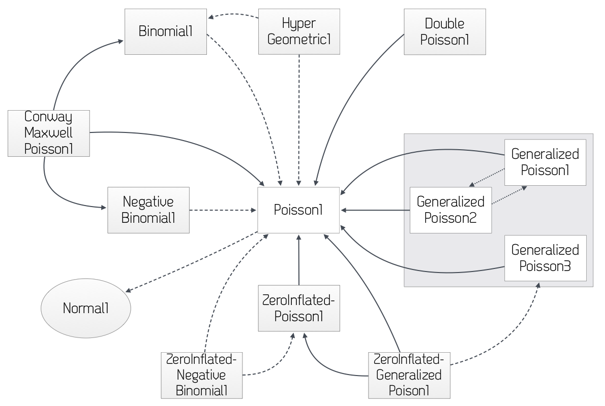
Figure 4.1: ProbOnto Poisson distributions

4.12.2.2 Binary data

Similar to count data above, we define the binary outcome and its distribution in a RANDOM_VARIABLE_DEFINITION block at the observation level of variability. Note how we define the names of the categories on the left hand side, and then the probability distribution defines the likelihood of the second category.

RANDOM_VARIABLE_DEFINITION(level=DV){
  Y withCategories {<category1>,<category2>} 
     ~ <ProbOnto distribution e.g. Bernoulli | Binomial>
}

For example (again, showing the INDIVIDUAL_VARIABLES, MODEL_PREDICTION and OBSERVATION blocks to show the model construction):

RANDOM_VARIABLE_DEFINITION(level=ID){
  eta_PPV_EVENT ~ Normal(mean=0, var=PPV_EVENT )
}# end RANDOM_VARIABLE_DEFINITION

INDIVIDUAL_VARIABLES{
  indiv_BASE : {type is linear, pop= POP_BASEP,
  ranEff=[eta_PPV_EVENT], trans is logit}
}# end INDIVIDUAL_VARIABLES

MODEL_PREDICTION{
  LP = logit(indiv_BASE) + POP_BETA\*CP
  P1 = invLogit(LP)
}# end MODEL_PREDICTION

RANDOM_VARIABLE_DEFINITION(level=DV){
  Y withCategories {none, event} ~ Bernoulli1(probability=P1)
}

OBSERVATION{
  :: {type is discrete, variable = Y }
}# end ESTIMATION

Note that the INDIVIDUAL_VARIABLES block defines the individual baseline by combining the population parameter and the random effect. Note also that this specification uses a logit transformation to ensure that the individual baseline indiv_BASE variable is on the (0,1) probability scale. Then, the linear regression with plasma concentration (CP) is defined in the MODEL_PREDICTION – Note that CP is not a covariate. Finally LP is back-transformed to the probability scale to give variable P1 which is the probability of an event to be used in the Bernoulli distribution. By defining how the 0,1 in the data correspond to named events {none, event} it is easier to understand exactly what category is being modelled.

An alternative distribution for the same model is the Binomial distribution with one trial:

RANDOM_VARIABLE_DEFINITION(level=DV){
  Y withCategories {none, event} ~ Binomial1(numberOfTrials=1, probability=P1)
}

OBSERVATION{
  :: {type is discrete, variable = Y }
} # end of OBSERVATION

4.12.2.3 Categorical data

Again, similar to count and binary data, the syntax for Categorical data outcomes is:

RANDOM_VARIABLE_DEFINITION(level=DV){
<variable> withCategories{ <category1>, …, <categoryk> } 
          ~ <ProbOnto distribution for categorical data
          e.g. CategoricalNonordered1 | CategoricalOrdered1>
}

OBSERVATION{
  :: {type is categorical, variable=<variable>}
}

For example (UseCase13_1):

GROUP_VARIABLES{
  B0 = Lgt0
  B1 = B0 + Lgt1
  B2 = B1 + Lgt2
}

INDIVIDUAL_VARIABLES{
  indiv_B0 : {type is general, grp = B0, ranEff = eta_PPV_EVENT}
  indiv_B1 : {type is general, grp = B1, ranEff = eta_PPV_EVENT}
  indiv_B2 : {type is general, grp = B2, ranEff = eta_PPV_EVENT}
}# end INDIVIDUAL_VARIABLES

MODEL_PREDICTION{
  EDRUG = Beta * CP
  A0 = indiv_B0 + EDRUG
  A1 = indiv_B1 + EDRUG
  A2 = indiv_B2 + EDRUG
  P0 = invLogit(A0)
  P1 = invLogit(A1)
  P2 = invLogit(A2)
  Prob0 = P0
  Prob1 = P1 - P0
  Prob2 = P2 - P1
  Prob3 = 1 - P2
} # end MODEL_PREDICTION

RANDOM_VARIABLE_DEFINITION(level=DV){
  Y withCategories{ none, mild, moderate, severe } 
      ~ CategoricalOrdered1(categoryProb=[Prob0, Prob1, Prob2, Prob3])
}

OBSERVATION{
  :: {type is categorical, variable=Y}
}

In the above code, the cutpoints between categories are defined in the GROUP_VARIABLES block (B0, B1, B2) and individual values for these are defined in the INDIVIDUAL_VARIABLES block. The linear effect of CP (plasma concentration) is defined in the MODEL_PREDICTION block and this is added to the individualised cutpoints (A0, A1, A2). These are then back-transformed to the probability scale (P0, P1, P2) and the ordered categorical model is defined by calculating the probability of each category as the difference from the previous category – Prob0, Prob1, Prob2, Prob3.

4.12.3 Time to event data

Time to event (TTE) models are modelled by specifying the hazard function. The PharmML to target software tool converters handle the translation of the hazard specification to target tool implementation. For some software this involves calculation of the survival function and associated likelihood.

For an arbitrary hazard function \[\lambda\left(t\right)\]:

Hazard function	\[\lambda\left( t \right)\]
Cumulative hazard function	\[\Lambda\left( a,\ b \right) = \ \int_{a}^{b}{\lambda\left( t \right)\text{dt}}\]
Survival function	\[P\left( T > t \right) = e^{- \Lambda\left( t_{0},t \right)}\]
Probability density function	\[p\left( t \right) = \lambda\left( t \right)e^{- \Lambda\left( t_{0},t \right)}\]
Cumulative distribution function	\[P\left( T < t \right) = \int_{0}^{t}{p\left( s \right)\text{ds}}\]

For an introduction to TTE models see (Holford 2013) and for a tutorial in implementation in NONMEM and Monolix see (N. H. M. Lavielle 2011).

The MDL syntax for time to event outcomes is :

<OUTCOME VARIABLE NAME> : { type is tte, hazard = <VARIABLE> }

For example (UseCase14.mdl):

INDIVIDUAL_VARIABLES{
  BTATRT = POP_BTATRT
  H_BASE = POP_HBASE
}

MODEL_PREDICTION{
  HBASE=H_BASE/365
  HAZTRT=BTATRT * TRT
  HAZ = HBASE * (1+HAZTRT)
} # end MODEL_PREDICTION

OBSERVATION{
  Y : {type is tte, hazard = HAZ }
} # end ESTIMATION

In the above case the hazard and the effect of treatment on the hazard is calculated in the GROUP_VARIABLES block. This is then used in the MODEL_PREDICTION block to calculate the hazard for the event. The model outcome variable Y is then defined as having type tte and the hazard calculated in the MODEL_PREDICTION block is passed in as an argument. Specification of the model is then very simple for the user – no calculation of Survival functions nor likelihood is necessary.

In the current MDL, TTE models are able to be handled equally by NONMEM and Monolix. To facilitate this, we impose certain constraints on dataset conventions. There must be a data record at the start of the interval during which the hazard will be integrated. We use DV = 0 to denote right censoring and DV = 1 to denote an event.

Currently only exact time of event and right censoring is supported in MDL. Future versions will support interval censoring and repeated time to event.

The convention in NONMEM datasets of using MDV to identify the start of the observation period for assessing TTE cannot be used.

4.13 `FUNCTIONS`

This block allows users to define their own functions, for example for use with interpolation.

The syntax is as follows:

<function name> :: function(<argument1> :: <argument1 type>,
    <argument2> :: <argument2 type>,
    <argumentk> :: <argumentk type>) :: <function result type>
    is
      <expression using argument1… argumentk>

Specifying the types of each argument and the type of the function result allows validation of the function inputs and outputs.

To call the function, the user types & before the function name.

For example:

FUNCTIONS{ myInterp::function(t::real, x0::real, t0::real, x1::real,
            t1::real)::real 
            is
              x0
 }

DATA_INPUT_VARIABLES {
  ID : { use is id }
  TIME : { use is idv }
  WT : { use is covariate, interp=&constInterp }
  AGE : { use is covariate, interp=&myInterp }
  }

4.14 `POPULATION_PARAMETERS`

The POPULATION_PARAMETERS block allows the user to define models and model parameters that exist at the population level. This may be used in hierarchical models to define population parameters when there are additional levels of hieararchy above the individual.

In most “population approach models, the individuals are assumed to be drawn from a population, the characterstics of which are described through fixed and random effect models. Inferences are then made on the “population parameters which we take to be representative of the population from which the individuals are drawn.

In meta-analysis across many studies, regions, demographic populations it may be useful to characterise additional levels of hierarchy characterising how individuals within each study, region or demographic differ systematically (through fixed effect models) and randomly (through variability models). These higher level models can be expressed in the POPULATION_PARAMETERS block.

In the current MDL, population models are defined through combination of RANDOM_VARIABLE_DEFINITION and POPULATION_PARAMETERS definitions. In the current MDL expressions (equations) are NOT allowed in the POPULATION_PARAMETERS block.

The POPULATION_PARAMETERS block uses random variables defined in the RANDOM_VARIABLE_DEFINITION block. The syntax for the POPULATION_PARAMETERS block is as follows:

POPULATION_PARAMETERS{
  :: {type is < continuous | categorical >, 
      variable = < RANDOM_VARIABLE_DEFINITION variable > }
}

For example (/FourModels/Hierarchical_Model.mdl):

RANDOM_VARIABLE_DEFINITION(level=POP){
  w_pop ~ Normal(mean = ws, sd = gw)
  V_pop ~ Normal(mean = Vs, sd = gV)
} # end RANDOM_VARIABLE_DEFINITION


POPULATION_PARAMETERS{
:: {type is continuous, variable=w_pop}
:: {type is continuous, variable=V_pop}
}

RANDOM_VARIABLE_DEFINITION(level=ID) {
  ETA_BSV_V ~ Normal(mean = 0, sd = omega_V)
  } # end RANDOM_VARIABLE_DEFINITION

INDIVIDUAL_VARIABLES {
  V : {type is linear, trans is ln, pop=V_pop, 
       fixEff={coeff=BETA_WT, cov=WT}, ranEff=ETA_BSV_V}
  } # end INDIVIDUAL_VARIABLES

MODEL_PREDICTION {
  D
  f = D/V * exp(-k*T)
  } # end MODEL_PREDICTION

In the model above, the mean weight for each population is drawn from a Normal random variable. The mean Volume of distribution also varies for each population and is similarly drawn from a Normal random variable. The parameters for inference would be Vs (“global mean of Volume of distribution), gV (between population variability), omega_V (between individual variability), BETA_WT (fixed effect of Weight). V_pop gives the population prediction of Volume of distribution for each population observed in the data, while V gives the individual predicted Volume of distribution.

References

Gelman, Andrew. 2006. “Prior Distributions for Variance Parameters in Hierarchical Models(Comment on Article by Browne and Draper).” Bayesian Analysis 1. Institute of Mathematical Statistics: 515–34. doi:10.1214/06-ba117a.

Swat, Maciej J., Pierre Grenon, and Sarala Wimalaratne. 2016. “ProbOnto: Ontology and Knowledge Base of Probability Distributions.” Bioinformatics 32 (17). Oxford University Press (OUP): 2719–21. doi:10.1093/bioinformatics/btw170.

Holford, Nick. 2013. “A Time to Event Tutorial for Pharmacometricians.” CPT: Pharmacometrics & Systems Pharmacology 2 (5). Wiley-Blackwell: e43. doi:10.1038/psp.2013.18.

Lavielle, Nick Holford; Marc. 2011. “A Tutorial on Time to Event Analysis for Mixed Effect Modellers.” http://www.page-meeting.org/pdf_assets/2573-time-to-event-tutorial.pdf.

4 Model Object

4.1 On interoperability

4.2 IDV

4.3 COVARIATES

4.4 STRUCTURAL_PARAMETERS

4.5 VARIABILITY_PARAMETERS

4.5.1 Residual Unexplained Variability

4.6 VARIABILITY_LEVELS

4.7 GROUP_VARIABLES

4.7.1 Defining model constants

4.8 RANDOM_VARIABLE_DEFINITION

4.9 INDIVIDUAL_VARIABLES

4.9.1 Mixed effect model with linear fixed effects and normally distributed

4.9.2 General mixed effect model with Gaussian random effects.

4.9.3 Mixed effect model defined by equations

4.9.4 INDIVIDUAL_VARIABLES without inter-individual variability

4.9.5 INDIVIDUAL_VARIABLES where the variable is defined in the

4.9.6 Conditional assignment of INDIVIDUAL_VARIABLES

4.9.7 INDIVIDUAL_VARIABLES definitions in practice.

4.10 MODEL_PREDICTION

4.10.1 DEQ

4.10.2 On Tlag and Bioavailability

4.10.3 COMPARTMENT

4.10.3.1 Input & absorption

4.10.3.2 Distribution processes

4.10.3.3 Elimination and transfer processes

4.11 Combining COMPARTMENT and DEQ blocks

4.12 OBSERVATION

4.12.1 Continuous outcomes

4.12.2 Discrete data

4.12.2.1 Count data

4.12.2.2 Binary data

4.12.2.3 Categorical data

4.12.3 Time to event data

4.13 FUNCTIONS

4.14 POPULATION_PARAMETERS

References

4.2 `IDV`

4.3 `COVARIATES`

4.4 `STRUCTURAL_PARAMETERS`

4.5 `VARIABILITY_PARAMETERS`

4.6 `VARIABILITY_LEVELS`

4.7 `GROUP_VARIABLES`

4.8 `RANDOM_VARIABLE_DEFINITION`

4.9 `INDIVIDUAL_VARIABLES`

4.9.5 `INDIVIDUAL_VARIABLES` where the variable is defined in the

4.9.6 Conditional assignment of `INDIVIDUAL_VARIABLES`

4.9.7 `INDIVIDUAL_VARIABLES` definitions in practice.

4.10 `MODEL_PREDICTION`

4.10.1 `DEQ`

4.10.3 `COMPARTMENT`

4.11 Combining `COMPARTMENT` and `DEQ` blocks

4.12 `OBSERVATION`

4.13 `FUNCTIONS`

4.14 `POPULATION_PARAMETERS`